Chapter 1

Chapter 1. Fundamentals

1.1 Moist thermodynamics 2/20

(Ref. 4, /chapter_4_Moist thermodynamic processes/4.4)

Moisture variables

Density (r_v, r_d)

Water vapor mixing (r): mass of water vapor per unit mass of dry air, r = r_v/r_d

Specific humidity (q): mass of water vapor per unit mass of air (including the vapor)

Vapor pressure (e or p_v)

Partial pressure of dry air (p_d)

Dalton’s law: p=e+ p_d

R_d : the weighted mean gas constant for all the constituents of air other than water vapor

R_v : the gas constant for water vapor

Relative humidity (RH): the ratio between the actual and saturation vapor pressure = e / e^*

r = r_v/r_d= R_d/R_v e / (p-e), where e = R_d/ R_v

q = r_v/ (r_d+ r_v) = r / (1+r)

Saturation values, r^*, q^*, e^*

Liquid water mixing ratio (r_l)

Ice mixing ration (r_i)
　

Thermodynamics of unsaturated moist air

The effective heat capacities of moist air are influence by the presence of water vapor.

Assuming the water vapor molecule is in the ground state

C_vv = 3 R_v = 1384.53 J kg^-1 K^-1

C_pv = 4 R_v = 1846.04 J kg^-1 K^-1

Over the range of tropospheric conditions

C_vv ~ 1410 J kg^-1 K^-1

C_pv ~ 1870 J kg^-1 K^-1

First thermodynamic law and second thermodynamic law: dQ = dU + pdV

Closed system and Open system

C_v^¢ º (¶Q/¶T)_v ~ C_vd (1+0.94r)

C_p^¢ º (¶Q/¶T)_p ~ C_pd (1+0.85r)

dQ = C_v^¢ dT + pda

dQ = C_p^¢ dT - a dp

specific volume: a º R^¢T / p

In adiabatic process, d lnT = (R^¢/C_p^¢ ) dlnp
　

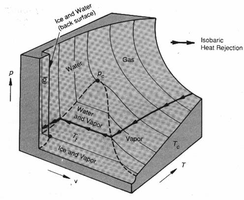
Phase equilibrium of water substance

The discussion above focuses on a homogeneous system, where only a single phase is present. For such a system, thermodynamic equilibrium requires mechanical and thermal equilibrium: no pressure and temperature difference between the system and its environment. For a heterogeneous system, wherein multiple phases are present, thermodynamic equilibrium also requires chemical equilibrium: no diffusion of mass from one phase to another.

The phase equilibria of water substance are determined by requiring

T_i= T_ii , p_i= p_ii , g_i= g_ii

where g is the Gibbs free energy: g º u + pa - Ts = k - Ts, s is the specific entropy,

k is the enthalpy: k º u + pa.

For a reversible, infinitesimal change while maintaining equilibrium,

dg_i = dg_ii,

Since dg = du + p da + a dp - Tds- sdT, and Tds = du+ p da (first law of thermodynamics)

a_idp-s_idT = a_iidp-s_iidT ® (dp/dT)_i,_ii = (s_ii- s_i)/(a_ii- a_i)

The latent heat pertaining to the phase transition of a substance is defined as

L_i,_ii º (k_ii- k_i) = T(s_ii- s_i)

(dp/dT)_i,_ii = L_i,_ii / T(a_ii- a_i)

This is the Clausius-Clapeyron equation

State surface for a (single-component) mixture of water involving multiple phases in equilibrium with one another. Thermodynamic process accompanying isobaric heat rejection also indicted.

Glaciers move (freezing decreases with increasing pressure)

r_ice > r_water
　

Clausius-Clapeyron Equation 2/20

, ,

1) Water-vapor equilibrium

2) Ice-vapor equilibrium

3) Ice-water equilibrium

, but

Home work 1 (due 3/13):

From the Clausius-Clapeyron Equation, ,

and the integrated Kirchhoff equation, ,

derive the above equations for , , and -1.344x10⁵ mb K^-1.

Also plot e^*(T).

Bergeron-Findeisen effect (Wegner- Bergeron-Findeisen)

Limitations of Clausius-Clapeyron Equation in cloud microphysics

Conserved moist thermodynamic variables

1.2 Clouds and microphysics

Characteristics and classification of clouds (student exercise)

Refer to Chapter 1: Identification of Clouds,

Houze, R. A. Jr., 1993: “Cloud dynamics”, Academic Press.

Homework 2 (due 3/20): translate description of clouds into English

Types of microphysical processes

Nucleation of particles

homogeneous and heterogeneous nucleation

Vapor diffusion

condensation, evaporation, deposition, and sublimation

Collection

continuous & stochastic coalescence, aggregation, riming, hail

Breakup of drops

Fallout

fall speeds of water drops and ice particles

Ice enhancement

several hypothesized processes

Melting

Refer to Chapter 3: Cloud microphysics,

Houze, R. A. Jr., 1993: “Cloud dynamics”, Academic Press.

1.3 Radiation 10/4

Refer to chapter_3: Atmospheric Radiative transfer and climate (3.1 to 3.8)

Dennis L. Hartmann, 1994: "Global Physical Climatology", Academic Press.

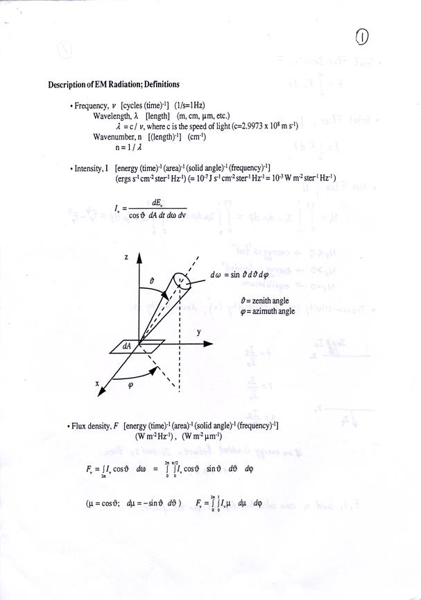
˙Total Flux Density, F

F = Fd

˙Total Flux,f

f=dA

˙Net Flux, N

N=Idd=Idd-Idd=F-F

N< 0 → energy is “lost”

N> 0 → energy is “added”

N= 0 → equilibrium

˙Transmissivity (t), Reflectivity (r), Absorptivity (a)

t =

r =

a =

If no energy is added between Z₀ and Z₁ then:

t + r + a = 1

t₁r₁ and a can also be defined for the fluxes.

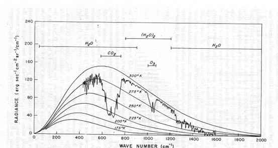
The terrestrial infrared spectra and various absorption bands. Also shown is an acture atmospheric emission spectrum taken by the Nimbus IRIS instrument near Guam at 15.1° N and 215.3°W on April 27, 1972.

Spectral irradiance distribution curves related to the sun; (1) the observed solar irradiance at the top of the atmosphere, and (2) solar irradiance observed at sea level. The shaded area represent absorption due to various gases in a clear atmosphere.

3/6 Home work (due 3/20)

Planck function:

B_l(T) = 2 h n³/ [c²(exp(hn/KT)-1], h=6.6262x10^-27 erg sec, K=1.3806x10^-16 erg deg^-1.

= 2 h c²/ l⁵ [c²(exp(hc/KlT)-1

Plot the plank function and derive the Stefan-Boltzmann Law (hint, x= hc/KlT

Interactions between em-radiation and matter

Matter in the atmosphere:

— gas molecules

N₂ (78 %)

O₂ (21 %)

CO₂ (0.03 %)

H₂O (0 ~ 0.04 %)

O₃ (0 ~ 1210^-4 %)

others (10^-4 ~ 10^-9 %)

— aerosol

— cloud (water droplets, ice crystals)

Interactions:

— Scattering: only part of the e.m.-radiation travels in the original direction, some appear in directions other than the original one.

I_s ~ k_sI₀dw

I_s(q) dw’ ~ k_sdw’ I₀dw

I_s = I_s(q) dw’

p(q) dw’ = 1

Types of scattering

Scattering depends on:

— chemical composition of the particle

— size of the particle, d

— wavelength of the incident radiation (λ)

1) d << λ → Rayleigh scattering (molecules)

k_s ~ λ^-4 (explains the blue color of the sky)

2) d λ → Mie scattering (aerosol, cloud)

— Absorption: some of the e.m. energy is converted into a different form of energy, e.g. kinetic energy, heat.

Measure: mass absorption cross section, k_a

[area (mass)^-1] (cm²g^-1)

— Molecules

Energy forms of a molecule:

E_total= E_{translational}+ E_rotational+ E_vibrational+ E_electronic

E_v = nhv

h = 6.62510^-34 Js

(Planck constant)

Example: energy levels for electronic transitions:

文字方塊: …...

Another way of describing e.m. radiation: consists of discrete amounts of energy called photons, E_v = hv

Absorption occurs if the energy of incident photon has an energy equal to the difference between two energy levels of the molecule. The molecule gets excited: E_i→E_j, j > i. When E_j→E_i, the molecule emits a photon with an energy of E=E_j-E_i. Since E is quantized, and equal to hv, the absorption and emission are selective.

Absorption and emission lines and line broadening

Broadening:

a) natural

b) pressure (collisions), Lorentz line shape

dominant in the troposphere

c) Doppler

Absorption/emission spectra: combination of lines corresponding to different energy levels of different transitions very complex structure → bands

Main absorption features in the atmosphere:

H₂O : triatomic molecule with permanent dipole moment →

— pure rotational band (l14 mm)

— strony vibration-rotation band at ~ 6.3mm

— several n/t bands between 0.8-4 mm

CO₂: linear symmetric molecule → no permanent dipole moment →

no pure rotational band

— strong n/t band ~15mm (peak of the terrestrial radiation)

— several other bands at 2, 3 and 4 mm

O₃: triatomic molecule

— strong n/t band at 9.6 mm

— weak band between 0.5-0.7 mm

N₂ and O₂: diatomic, symmetric molecules → no permanent dipole moment → no vibrational and simple rotational spectra.

Absorption and emission caused by electronic transitions. (high energy) → UV and visible spectra.

None or very weak absorption between 0.3-0.7 mm

Additional types of absorption

a) Photodissociation: breaking the bond between atoms.

Requires large energy → l < 0.2, 0.3 mm

b) Photoionization: removing electrons. Even larger energies are needed → l < 0.1 mm

Particles: energy levels are so complex, and so close to each other that absorption and emission is continuous.

Extinction) ke

k_e= k_a+ k_s

The Equation of Transfer (E.T.)

The change of energy is due to extinction and emission:

dI = -k_erdsI + jrds

= -I + y, y = : source function

Special case: assume y = 0

I(S₁) = I(0) e^- (Beer-Bouguer-Lambert Law)

Note: it is valid for fluxes too.

t = = e^-

E.T. for a plane-parallel atmosphere

Introducing the normal optical depth as d= -k_eρdz

m= I() - y()

Source function, y in Radiative Transfer Equation (RTE)

a) For multiple scattering:

jrds = rds(dw, dw’)I(dw’)dw’

y = (dw, dw’)I(dw’)dw’

→= single scattering albedo

y depends on I (!!!) no “easy” solution for RTE.

b) For thermal radiation:

jrds = rds : intensity of radiation emitted at a wave length l by the atmosphere (or surface) at temperature T.

=f(l, T) in thermodynamic equilibrium f(l, T) is the same for any substance (Kirchhoff’s Law)

for a “black body” a_l=1 f(l, T) is the emitted intensity of a black body, B_l(T)

= a_lB_l(T) → y=== (1-) B_l(T)

ke=1- e_l= emissivity

=a_l= e_l

e_l= a_l emissivity = absorptivity

B_l(T)= Planck’s Law h=6.6310^-34Js

k=1.3810^-23JK^-1

Properties of B:

— B_l(T) does not depend on direction (isotropic radiation)

— The wavelength of maximum emission is inversely proportional to the absolute temperature: l_max[mm]=

(Wien’s law)

(Source function, y contiuned)

Black body curves for solar and terrestrial temperatures

文字方塊: lBl (normalized)

Solar and terrestrial radiation can be treated separately

— total energy in a hemisphere (total flux density):

F==sT⁴ (Stefan-Boltzmann law)

s=5.6710^-8 Wm^-2K^-4

Solution of the RTE in a plane-parallel atmosphere

RET: m =I(τ;μ;φ)-y (τ;μ;φ)

I(τ;μ;φ)=I(τ₁;μ;φ)e^-(τ^1-τ)/μ+ e^{-(τ'-τ)/ μ}

I(τ_;-μ;φ)=I(0_;-μ;φ)e^-τ/μ+ e^{-(τ-τ')/ μ}

Total fluxes in the infrared (IR) spectrum (thermal flux)

1) Assume there is no scattering (=0) y= B_l(T)

2) Use transmissivity, t as a vertical coordinate in RTE instead of τ. t(z₁,z₂)=e

3) Calculate F()=

Upward flux at the top of the atmosphere (z=):

F^↑()=

Downward flux at the surface (z=z_s):

F^↓(z_s)= =

Plot of and T(z)

− the transmissivity between surface and top of atmosphere − is small. Only small amount of energy from the surface reaches the top

is large enough only for small values of z. Most of the flux F^↓ comes from the lower part of the atmosphere.

In an absorbing atmosphere:

1) energy loss by emission to space is much less

than the IR emission from the surface, “greenhouse” effect

2) there is a supply of downward flux from the

warm lower atmosphere

Emission temperature, T_e

F^↑()=→T_e= ≈ 255K or -18ºC

Radiative equilibrium temperatures

Assume:

—Solar radiation is absorbed at the surface only,

—The atmosphere is composed of layers which emit like, black bodies, they are opaque for IR radiation

—There is a balance of incoming and outgoing fluxes for each layer.

A_top=0.3 (planetary albedo)

S=1360Wm^-2 (solar constant)

Solution T₁=255K (=T_e)

T₂=303K

T_s=335K (observed mean Ts ≈ 288K (!)) there are physical processes other than radiation which transport heat away from the surface (convection, evaporation)

Fact: radiative equilibrium T(z)observed T(z) → do convective adjustment: kntical value (6.5 K km^-1). If >6.5K km^-1 assume a nonradiative upward heat transfer. is lapse rate.

Radiative-Convective Equilibrium Temperature (RCET) profiles

— Obtained from a steady balance solution of complex models.

The models include the following variables.

• H₂O

• CO₂

• O₃

• Aerosols

• Cloud

• Surface albedo

— RCET profiles approximate the global mean temperature profile of the Earth’s atmosphere.

Is the atmosphere-surface system in a radiative balance?

文字方塊: Remember!:N=F↓-F↑ Need to calculate or observe the net flux at the top of the atmosphere:

N_TOA=N_SW+N_LW=F(1- A_TOA)-σT SW: short wave

LW: long wave

N_TOA averaged over several years is zeroequilibrium.

On a monthly time scale N_TOA > 0 or N_TOA< 0.

What about the radiative balance at the surface?

N_SRF=N_SW+N_LW=F(1-A_SRF)-eσT+ F

Daytime: eσT≈ F the shortwave heating is dominant

At night: N_sw=0 and eσT> Fcooling

How does the temperature change in time?

Conservation of energy absorbed radiation is converted into heat

Absorbed radiation is ∆N=N(z+dz)-N(z) ——— z+∆z

∆N=c_pρ∆z ——— z

t: time

c_p: specific heat at constant pressure

: radiative heating rate

Radiative heating rate profile

< 0 cooling (in the longwave spectrum)

> 0 warming (in the shortwave spectrum)

In the stratosphere LW cooling by CO₂ is compensated by SW warming by O₃.

In the troposphere LW cooling by CO₂ is balanced by SW warming by H₂O. LW cooling by H₂O is balanced by nonradiative processes (convective heat transfer from the surface). (H₂O is the most important greenhouse gas.)

Effect of clouds on N_TOA and N_SRF

Net (SW+LW)

TOA

increase A_TOA

decrease N_SW

cooling

decrease T_e

increase N_LW

warming

cooling/warming

Surface

decrease F

decrease N_SW

cooling

increase F

increase N_LW

warming

cooling/warmin

Cloud forcing, CF

CF = N_all-sky– N_clear-sky

In SW: N_all-sky < N_clear-sky CF_SW< 0 → cooling

In LW: N_all-sky > N_clear-sky CF_LW> 0 → warming

In the tropics CF ≈ 0

At high latitudes CF < 0