Chapter 11 Quantum physics: introduction
Contents
- Blackbody radiation
- Photoelectric effect
- Compton effect
- Wave properties of a particle and de Broglie's matter wave hypothesis
- A new model of a quantum particle
- Heisenberg's uncertainty principle
- Probability interpretation of matter waves
- Schrodinger's equation
- Brief review of atomic physics
- Exercises
$\S$ Black-body radiation
In mid-19th century, people realized that the spectrum of radiation from warm objects seemed to be universal and only depended on the temperature. Such radiation is called thermal radiation, and then black-body radiation due to historical reasons of the scientific development.
Why black-body? In thermal equilibrium, the spectrum of thermal radiation from an object must be equal to the spectrum of absorption. Otherwise, the object would heat up or cool down because of imbalance of radiation energy input and output. Therefore, a perfect radiator must be also a perfect absorber, which must appear black for the whole spectral range.
A good approximation of a black body is a small hole leading to the inside of a hollow object. The nature of the radiation leaving the cavity through the hole depends only on the temperature of the cavity walls. The EM radiation emitted is called blackbody radiation.

- There are two features of this distribution: A. The total power of the emitted radiation increases with temperature, according to Stefan’s Law: $$P=\sigma A e T^4,$$where $e=1$ for a perfect black body, $A$ is the area of the surface. The Stephan-Boltzmann's constant $\sigma=5.67\times 10^{-8}$ W/(m$^2\cdot$ K$^4$). B. The peak of the wavelength distribution shifts to shorter wavelengths as the temperature increases according to Wien’s displacement law: $$\lambda_{max}T = 2.898\times 10^{-3} \text{m}\cdot\text{K},$$ where $\lambda_{max}$ is the wavelength at which the curve peaks, and $T$ is the absolute temperature.

To describe the distribution of energy from a black body, we define $I(\lambda,T)d\lambda$ to be the intensity, or power per unit area, emitted in the wavelength interval $d\lambda$.
In the classical theory, the black-body radiation is caused by charged oscillators of the cavity walls as they are accelerated and emit EM waves at all wavelengths. The average energy for each wavelength of the standing-wave modes is assumed to be proportional to $k_B T$, based on the theorem of equipartition of energy, leading to the Rayleigh–Jeans law: $$I(\lambda,T)=\frac{2\pi ck_B T}{\lambda^4}.$$
At short wavelengths, there was a major disagreement between classical theory and experimental results for black body radiation. This mismatch became known as the ultraviolet catastrophe. You would have infinite energy as the wavelength approaches zero.
In 1900, Planck developed a structural model for blackbody radiation that leads to an equation in agreement with the experimental results. His model represents the dawn of quantum physics!
Planck's theory
The energy of the oscillator is quantized; that is, it can have only certain discrete amounts of energy $E_n$ given by $E_n = nhf$, where $n$ is a positive integer called the quantum number, $h$ is Planck’s constant, $ƒ$ is the frequency of oscillation. This says the energy is quantized.
Each discrete energy value corresponds to a different quantum state, represented by the quantum number $n$. An oscillator radiates or absorbs energy only when it makes a transition from one energy state to a different state.
Planck formula: $$I(\lambda,T)=\frac{2\pi hc^2}{\lambda^5(e^{hc/(\lambda k_B T)}-1)}.$$
The Planck constant $h=6.625\times 10^{-34}$ J$\cdot$s.
We do not see quantum effects on an everyday basis because the energy change in a macroscopic system due to a transition between adjacent states is such a small fraction of the total energy of the system that we could never expect to detect the change. Our senses perceive the increase and decrease as continuous.
Quantum effects become important and measurable only on the submicroscopic level of atoms and molecules.
Quantum results must blend smoothly with classical results when the quantum number becomes large. This statement is known as the correspondence principle.
Derivation of Rayleigh-Jeans law and Planck's hypothesis (Optional)
Since the intensity density $I(\lambda,T) \propto u(\lambda,T)c$, where $u(\lambda,T)$ is the energy-density density. That is, $u(\lambda,T)d\lambda$ is the energy density, defined as energy per unity volume, contributed to by modes within ($\lambda$,$\lambda+d\lambda$).
- It is actually $I=\frac{1}{4}uc$. The factor $\frac{1}{4}$ comes from only one half of the standing waves entering the half-space where the hole is, and one half from projecting the radiation direction onto the one towards the hole.
Our strategy:
To count the number of modes within ($\lambda$,$\lambda+d\lambda$).
To calculate the averaged energy carried by each mode.
Calculate $u(\lambda,T)=$ (# of modes within $\lambda$ and $\lambda+d\lambda$)$\times$(expected energy for that mode).
Counting the number of modes
To do that, consider a cubic cavity of side length $L$. The allowed standing wave modes are of the form $$ E\propto\sin k_{n_x}x\sin k_{n_y}y\sin k_{n_z}z,$$ where $k_{n_{x,y,z}}=n_{x,y,z}\pi/L$. Each tuple $(k_{n_x},k_{n_y},k_{n_z})$ determines a mode. The overall wave number is $k_{(n_x,n_y,n_z)}=\sqrt{k_{n_x}^2+k_{n_y}^2+k_{n_z}^2}=\frac{\pi}{L}\sqrt{n_x^2+n_y^2+n_z^2}$. By definition, $k=2\pi/\lambda$. For a specific $\lambda$, it corresponds to a specific $k_n$ with $n\equiv\sqrt{n_x^2+n_y^2+n_z^2}$.
These $(n_x,n_y,n_z)$ correspond to grid points in the first octant. By treating the distribution a continuum approximately, the number of grid points within a radius $n$ in the first octant is $\frac{1}{8}\frac{4}{3}\pi n^3$. And the number of grid points within $n$ and $n+dn$ is $$\frac{1}{2}\pi n^2dn.$$ Also, since $n=\frac{2L}{\lambda}$ and then $|dn|=\frac{2L}{\lambda^2}d\lambda$, and each mode can have two independent polarizations, the total number of modes within $\lambda$ and $\lambda+d\lambda$ is $$ 2\times \frac{1}{2}\pi \left(\frac{2L}{\lambda}\right)^2 \left(\frac{2L}{\lambda^2}d\lambda\right)=\frac{8\pi L^3}{\lambda^4}d\lambda. $$
Finding the expected energy
Classical prediction: Using the theorem of equipartition of energy, each mode corresponds to $k_B T$. Then we multiply the number of modes by $k_B T$ and divide it by $V=L^3$, and we get $$u(\lambda,T)=\frac{8\pi k_B T}{\lambda^4}$$and $$I(\lambda,T)=\frac{2\pi ck_B T}{\lambda^4}.$$ This is Rayleigh-Jeans's law.
Planck's hypothesis: For each mode, the energy excitation and de-excitation must be done by exchanging a quantum of energy $E=hf$. So for this mode in the thermal equilibrium, its actual state is a probabilistic combination: in the state of $n$ quanta (therefore $E_n=nhf$) with a probability $p_n$.
From Boltzmann relation $p_n\propto e^{\frac{-E_n}{k_B T}}$. This probability must be appropriately normalized. We calculate $$ Z=1+e^\frac{-E}{k_B T}+e^\frac{-2E}{k_B T}+e^\frac{-3E}{k_B T}+\cdots=\frac{1}{1-e^\frac{-E}{k_B T}} $$ so $$ p_n=\frac{e^\frac{-nhf}{k_B T}}{Z}. $$ Note that $f=c/\lambda$.
We then calculate the averaged energy for this mode by $\langle E\rangle=\sum_n p_n nhf=\frac{hc}{\lambda\left(e^\frac{hc}{\lambda k_B T}-1\right)}.$ Then $$u(\lambda,T)=\frac{8\pi hc}{\lambda^5\left(e^\frac{hc}{\lambda k_B T}-1\right)}$$ and $$I(\lambda,T)=\frac{2\pi hc^2}{\lambda^5(e^{hc/(\lambda k_B T)}-1)}.$$ This is Planck's results.
$\S$ Photoelectric effect

The photoelectric effect occurs when light incident on certain metallic surfaces causes electrons to be emitted from those surfaces. The emitted electrons are called photoelectrons. The effect was first discovered by Hertz.
The current arises from photoelectrons emitted from the negative plate (E) and collected at the positive plate (C). The current increases as the intensity of the incident light increases. When $\Delta V$ is negative, the current drops because many of the photoelectrons emitted from E are repelled by the negative collecting plate C.
Dependence of photoelectron kinetic energy on light intensity:
[Classical Prediction] Electrons should absorb energy continually from the electromagnetic waves. As the light intensity incident on the metal is increased, the electrons should be ejected with more kinetic energy.
[Experimental Result] The maximum kinetic energy is independent of light intensity. The current goes to zero at the same negative voltage for all intensity curves.
- Time interval between incidence of light and ejection of photoelectrons
[Classical Prediction] For very weak light, a measurable time interval should pass between the instant the light is turned on and the time an electron is ejected from the metal. This time interval is required for the electron to absorb the incident radiation before it acquires enough energy to escape from the metal
[Experimental Result] Electrons are emitted almost instantaneously, even at very low light intensities. (Less than $10^{-9}$ s.)
- Dependence of ejection of electrons on light frequency
[Classical Prediction] Electrons should be ejected at any frequency as long as the light intensity is high enough.
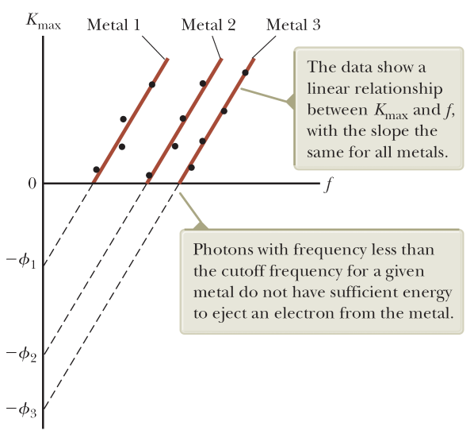
[Experimental Result] No electrons are emitted if the incident light falls below some cutoff frequency $ƒ_c$. The cutoff frequency is characteristic of the material being illuminated. No electrons are ejected below the cutoff frequency regardless of intensity.
- Dependence of photoelectron kinetic energy on light frequency
[Classical Prediction] There should be no relationship between the frequency of the light and the electric kinetic energy. The kinetic energy should be related to the intensity of the light.
[Experimental Result] The maximum kinetic energy of the photoelectrons increases with increasing light frequency.
Einstein's model: A photon of incident light gives all its energy $hƒ$ to a single electron in the metal. The absorption of energy by the electrons is a discontinuous process in which energy is delivered to the electrons in bundles.
The system has two types of energy: the potential energy of the metal–electron system and the kinetic energy of the ejected electron. According to the conservation of energy equation $$\Delta K + \Delta U = T_{ER}.$$ The energy gained by an photoelectron must overcome the potential called the work function $e\phi$ of the metal, and the maximal kinetic energy is given by $K_{max}=hf-e\phi$, which was predicted by Einstein and then has been demonstrated later.
If the energy of an incoming photon does not satisfy this requirement, an electron cannot be ejected from the surface, even though many photons per unit time are incident on the metal in a very intense light beam.
$\S$ Campton effect: Scattering of X-rays

[Classical theory]
- According to the classical theory, electromagnetic waves of frequency $ƒ_0$ incident on electrons should accelerate in the direction of propagation of the x-rays by radiation pressure, and oscillate at the apparent frequency of the radiation since the oscillating electric field should set the electrons in motion. Overall, the scattered wave frequency at a given angle should be a distribution of Doppler-shifted values.
[Experiment result]
- Compton’s experiments: The x-rays, scattered from a carbon target, were diffracted by a rotating crystal spectrometer, and the intensity was measured with an ionization chamber that generated a current proportional to the intensity. The incident beam consisted of monochromatic x-rays of wavelength $\lambda_0 = 0.071$ nm.

The experimental intensity-versus-wavelength plots observed by Compton for four scattering angles are shown in the figure. The graphs for the three nonzero angles show two peaks, one at $\lambda_0$ and one at $\lambda^\prime > \lambda_0$.
The scattering of x-ray photons from electrons could be explained by: treating photons as point-like particles with energy $hf$ and momentum $hf/c$ assuming that the energy and momentum of the isolated system of the photon and the electron are conserved in a two-dimensional collision.
Derivation:
Conservation of momentum: $$\vec p_0 = \vec p+\gamma m_e\vec v.$$ Conservation of energy: $$p_0 c+m_ec^2=p c+\gamma m_ec^2.$$
Note that $$(\vec p_0-\vec p)^2=(\gamma m_e v)^2=p_0^2+p^2-2pp_0\cos \theta.$$ Also, from $$p_0-p=\gamma m_e c-mc,$$ we have $$p_0^2+p^2+2pp_0=(\gamma-1)^2m^2c^2$$ and $$pp_0(1-\cos\theta)=(\gamma-1)m^2c^2=mc(p_0-p).$$ This leads to $$\lambda-\lambda_0=\frac{h}{mc}(1-\cos\theta).$$
$\S$ Wave properties of a particle and de Broglie's matter wave hypothesis
Light has a dual nature in that it exhibits both wave and particle characteristics. The particle model and the wave model of light complement each other.
In 1923, Louis de Broglie postulated that because photons have both wave and particle characteristics, perhaps all forms of matter have both properties. The relationship between energy and momentum for a photon is $p = E/c$; the energy of a photon is $E = hf = hc/\lambda$; the momentum of a photon can be expressed as $$p=\frac{E}{c}=\frac{hf}{c}=\frac{h}{\lambda}$$.
De Broglie suggested that material particles of momentum $p$ should also have wave properties and a corresponding wavelength given by the same expression. The de Broglie wavelength of a particle is $$\lambda=\frac{h}{mv}.$$ Its frequency is $$f=\frac{E}{h}.$$
In 1927, three years after de Broglie published his work, Davisson and Germer (US), and Thomson (England) succeeded in observing these diffraction effects and measuring the wavelength of electrons.
$\S$ A new model of a quantum particle
Particle-wave duality.
The locality of a particle can now be understood through the concept of a wave packet. A wave packet consists of waves of near frequencies that form a wave localized in space.
For instance:
%matplotlib notebook
import numpy as np
import matplotlib.pyplot as plt

xs=np.linspace(-1.,1,1001)

def nmode(f):
    return np.cos(f*2*np.pi*xs) # mode profiles

def ysf(df,f0): # f0 is central frequency and df is the frequency width
    ys=np.zeros(np.size(xs))
    for dw in np.linspace(-df,df,101):
        an=np.exp(-dw**2) # amplitudes of constituting modes
        ys=ys+an*nmode(f0+dw)
    return ys

plt.figure(figsize=(5,2))
plt.plot(xs,ysf(1.2,10))
plt.xlim(-1,1)
plt.grid(True)
plt.show()

Phase velocity $v_p=f\lambda=\frac{\omega}{k}$
Group velocity $v_g=\frac{\Delta \omega}{\Delta k}$. Why? Look at the two-mode example.
In the continuous limit: $v_g=\frac{d\omega}{dk=\frac{dE}{dp}}$.
For a free non-relavistic particle: $E=\frac{1}{2}mv^2$ and $p=mv$. The group velocity is $$v_g=\frac{mvdv}{mdv}=v.$$
$\S$ Heisenberg's uncertainty principle
- Coordinate-momentum undertainty relation: $$\Delta x\Delta p_x\ge\frac{\hbar}{2}.$$
Concept:
We inject a quantum particle through a single slit. The position uncertainty is determined by the slit size $\Delta x=a$. At the same time, it produces an uncertainty of the transverse momentum, such that the central maximum has a width determined by $\theta\sim \frac{\lambda}{a}$. Note that $\theta\sim \frac{\Delta p_x}{2p}=\frac{\Delta p_x\lambda}{2h}$. Therefore we get $\Delta x \Delta p_x \sim h$.
Estimation of the energy of a hydrogen atom
The size of a hydrogen atom is determined by the most probable radius $r$ through $\Delta x=r$. According to the unicertainty relation $p\sim \frac{\hbar}{r}$. The total energy is $$E_total=U+E_k=-\frac{ke^2}{r}+\frac{p^2}{2m}\sim -\frac{e^2}{4\pi\epsilon_0 r}+\frac{\hbar^2}{2mr^2}.$$ Minimization of this energy gives the Bohr radius $r\equiv a_0=\frac{4\pi\epsilon_0 \hbar^2}{me^2}$.
- Energy-time uncertainty relation: $$\Delta E\Delta t\ge \frac{\hbar}{2}.$$
To measure the frequency of a sinusoidal wave by observation for a period of time $\Delta t$, the measured phase must be within $\omega \Delta t\in 2\pi(N,N+1)$. The uncertainty of the frequency is $\Delta \omega =\frac{2\pi}{\Delta t}$. Then $$\Delta E\Delta t=\hbar\Delta \omega \Delta t\sim h.$$
$\S$ Probability interpretation of matter waves
Double-slit experiment for single electrons.
A matter wave can be described by a wavefunction $\psi(x)$, which should be understood as a probability amplitude. That is, the probability of finding a quantum particle within the space $(x,x+dx)$ is given by$$P(x)dx=|\psi(x)|^2dx$$ in 1D systems. Generalization to 3D is straightforward.
All probabilities add up to be 1. In 1D, $$\int_{\text{all allowed space}} |\psi(x)|^2dx=1.$$
The probability os finding a quantum particle within $x\in(a,b)$: $$\int_a^b |\psi(x)|^2dx=1.$$
A physical quantity is called an observable in quantum mechanics. The classical value of a physical quantity corresponds to the expectation value of the observable. For instance, $$ \langle \hat x\rangle =\int \psi^\ast x\psi dx. $$
Observables are actually (Hermition) operators in quantum mechanics. Not any two operators commute, i.e., they cannot change orders. These usually associate with an uncertainty relation between these operators, and also suggest they cannot be measured of arbitrary accuracy simultaneously.
The most important example: $\hat x$ and $\hat p_x$ do not commute $\hat x\hat p_x-\hat p_x \hat x\equiv[\hat x,\hat p]\neq 0$. Actually $$[\hat x,\hat p]=i\hbar.$$
Expectation value of $\hat p_x$
As $\hat p_x$ is also an observable, the classical value of $\hat p_x$ is $$\langle \hat p_x\rangle=\int \psi^\ast \hat p_x \psi dx=\int \psi^\ast \frac{\hbar}{i}\frac{d}{dx} \psi dx$$ or $$\hat p_x=\frac{\hbar}{i}\frac{d}{dx}.$$
Check (your homework): $$[\hat x,\hat p_x]=i\hbar.$$
A quantum particle in a box
Consider a 1D box of length $L$ containing a quantum particle of mass $m$. The wavefunction of $m$ should be formed by standing wave solutions within the box. So $$\phi_n(x)=A\sin\frac{n \pi}{L}x,$$ where $n=1,2,3,\cdots$ denotes the possible states of the particle.
Normalization of each state $\phi_n(x)$: From $$\int_0^L |\phi(x)|^2 dx=A^2\int_0^L \sin^2 \frac{n\pi}{L}x dx=1,$$ we get $A=\sqrt{\frac{2}{L}}$.
Since the wavelength of each mode $\phi_n$ is given by $\lambda_n=\frac{2L}{n}$, the momentum is $$p_n=\frac{h}{\lambda_n}=\frac{nh}{2L}.$$ (Note here $p_n$ is the magnitude of the matter-wave momentum, not $\langle p_x\rangle$, which is 0 because it is the expectation value of a 1D vector.)
The corresponding energy is $$E_n=\frac{p_n^2}{2m}=\frac{h^2}{8mL^2}n^2.$$
Note that the general solution is a superposition of $\phi_n(x)$: $$\psi(x)=\sum_n c_n \phi_n(x)$$ with $|c_n|^2$ the probability of finding the particle in state $\phi_n(x)$ and $\sum_n |c_n|^2=1$. Further, $$\langle E\rangle=\sum_n |c_n|^2 E_n.$$
Since these standing-wave solutions have well-defined energies and form a basis, we call $\phi_n$ the eigenstate, $E_n$ the eigenenergy, and the whole familty the eigenbasis.
$\S$ Schrodinger's equation
Matter waves follow Schrodinger's equation. In 1D, it reads $$ i\hbar\frac{\partial}{\partial t}\Psi(x,t)=-\frac{\hbar^2}{2m}\frac{\partial^2}{\partial x^2}\Psi(x,t)+U(x)\Psi(x,t).$$
For stationary solutions, one can write $\Psi(x,t)\sim\psi(x)e^{iEt/\hbar}$, where $E$ is the energy of the system. Then we have $$-\frac{\hbar^2}{2m}\frac{d^2}{d x^2}\psi(x)+U(x)\psi(x)=E\psi(x).$$
Example: A quantum particle in a box
Example: Tunneling
Derivation similar to the discussion of the reflection and transmission at the interface between different materials in the case of string waves.
The transmission coefficient: $$T\approx e^{-2CL},$$ where $L$ is the thickness of a rectangular barrier, and $C=\frac{\sqrt{2m(U-E)}}{\hbar}$ with $U$ the barrier height and $E$ the incident kinetic energy.
$\S$ Brief review of atomic physics
J. J. Thomson: A volume of positive charge with electrons embedded throughout the volume.
E. Rutherford: Planetary model
- Rutherford's foil experiment: A beam of positively charged alpha particles hit and were scattered from a thin foil target. Large observed deflections could not be explained by Thomson’s model.
- Positive charge is concentrated in the center of the atom, called the nucleus. Electrons orbit the nucleus like planets orbit the Sun.
- Difficulties: (a) Atoms emit certain discrete characteristic frequencies of electromagnetic radiation (b) Rutherford’s electrons are undergoing a centripetal acceleration. These should radiate electromagnetic waves of the same frequency. The radius should steadily decrease as this radiation is given off. The electron should eventually spiral into the nucleus, which does not occur.
N. Bohr: Stationary-orbit model
- Bohr postulated (a) electrons in atoms are generally confined to stable, nonradiating orbits called stationary states. These orbits are formed such that the electron's angular momentum is a multiple of $\hbar$, i.e., $$L_n=n\hbar$$ (b) The frequency of radiation emitted obeys $E_f-E_i=hf$ when the atom makes a transition from one stationary state i to another f.
- Difficulties: (a) It failed to predict more subtle spectral details. Many of the lines in the Balmer and other series were not single lines at all. Each was a group of closely spaced lines. Some single spectral lines were split into three closely spaced lines when the atoms were placed in a strong magnetic field. (b) No direct evidence for the existence of the stationary states.
- de Broglie's argument: Bohr's stationary-state (angular momentum is multiple of $\hbar$) conditions can be fulfilled by taking the electron's matter wave to form standing waves along the circular orbit: $$2\pi r_n=n\lambda_n,$$ $$L_n=r_n p_n=r_n \frac{h}{\lambda_n}=n\hbar.$$
- But this explanation is just a convenience. The true understanding of these states must rely on the interpretation of Schrodinger's wavefunctions.
The expected true theory must also have a duality: (a) The electron must have dynamical properties such as kinetic energy and momentum (wavelength). (b) The charge density must be stationary in time. Otherwise, it would radiate energy.
From solving Schrodinger's equation, we get these stationary states, which look like $$\Psi_n(\vec r,t)\sim \psi_n(\vec r)e^{-i\omega_n t}.$$ Note that $$|\Psi_n(\vec r,t)|^2=|\psi_n(\vec r)|^2,$$ where the charge density is stationary but in the same time the system contains an energy and momentum with the relation: $E_n=\hbar\omega_n=U(r_n)+\frac{p_n^2}{2m}$.
Consider a superposed state $\Psi(x,t)=c_1 \psi_1(x)e^{-i\omega_1 t}+c_2 \psi_2(x)e^{-i\omega_2 t}$. The magnitude (square) of the composite wavefunction is $$|\Psi|^2=|c_1|^2|\psi_1|^2+|c_2|^2|\psi_2|^2+2|c_1| |c_2| |\psi_1||\psi_2|\cos((\omega_1-\omega_2)t+\phi)$$ corresponding to charge density varying in time at a frequency $\Delta \omega$, explaining why the radiated frequency $\sim \hbar\Delta \omega=\hbar(\omega_1-\omega_2)=E_1-E_2$.
Unfortunately, we do not have enough time to talk about the hydrogen atom's solution to Schrodinger's equation though it is rather important to understand the periodic table and related topics in chemistry. Please refer to our textbook for the details.
$\S$ Exercises
Serway Textbook
Ch 28 Problems 1, 8, 13, 15, 17, 21, 23, 25, 27, 32, 39, 41, 42, 43, 47