Read NetCDF files (using NetCDF4 package)
NetCDF (.nc) 是大氣與地球科學界常用的一種檔案格式,同一個nc檔案中除了變數的資料數值,還儲存了該變數檔案格式(如維度大小、經緯度、時間、物理單位...)等重要資訊。使用正確的netCDF套件讀取.nc檔,就可以很方便地讀出這些重要的檔頭或metadata,不需要再參考額外的描述檔(如GrADS需要.ctl檔)
NetCDF (.nc) is a commonly used file format in atmospheric science and earth science. It is a self-describing file format, that is, the information about the dimension, geolocation coordinate, variable names, units...., are stored with the data values together inside the same file.
Reading the .nc file using correct netCDF library, one can obtain these "metadata" (latitude, longitude, time...etc) easily and use them in plotting figures or computation, without referring to a seperate describtion file or control file (such as GrADS .ctl)
Here we introduce the NetCDF4 package in python for dealing with the .nc files. NetCDF4 is available on study server. Some of you may not have NetCDF4 installed in the python system on your computer. (check this by "import NetCDF4"). To install, please see the steps here:http://homepage.ntu.edu.tw/~weitingc/fortran_lecture/Lecture_P_4_Installing_Basemap_NetCDF4.slides.html
Reference for NetCDF4 Package: http://unidata.github.io/netcdf4-python/
#跟其他套件一樣,我們必須先import進來
import netCDF4 as nc

# we also need these packages
import numpy as np  # processing data array
import matplotlib.pyplot as plt  # making plots
import datetime     # convert time to date format
1. 讀取nc檔
- 將檔頭存到rootgrp之後,顯示此變數可以看到一些有用的資訊,包括資料維度、格式、資料的說明等等
- 接著將需要的資料變數數值(如經緯度、溫度)存到指定的陣列名稱(型態是numpy.ndarray)
- 範例資料檔可以從study主機下載:/home/teachers/weitingc/hw/GFS20171217_tmp.nc
rootgrp = nc.Dataset("GFS20171217_tmp.nc")
rootgrp # show metadata information
 # first let's extract the lat, lon, and pressure level information and store as numpy arrays
lat = rootgrp.variables['lat'][:]
lon = rootgrp.variables['lon'][:]
lev = rootgrp.variables['lev'][:]
print(lat.shape)
# We can also get time information, and convert to calendar date
time = rootgrp.variables['time'][:] # get value of time
time_u=rootgrp.variables['time'].units # get unit
time_d=nc.num2date(time,units = time_u,calendar='standard') # get date using NetCDF num2date function
print(time)
print(time_u)
print(time_d)
# check the information about the variable tmp (temperature)
print(rootgrp.variables['tmp'])
2. 繪圖、運算
- 這邊將讀取到的溫度畫出做簡單的繪圖與運算,有四個例子:
- 畫出第一個time step, 經度120E, 緯度25N網格點的溫度垂直分布
- 畫出第一個time step, 850hPa的全球等溫線分布(參考2Dplot講義,要疊加地圖的範例請參考Basemap)
- 計算並畫出第二個time step, 緯向平均(zonal average)溫度剖面。
- 計算並畫出第二個time step, 經向平均(meridional average)溫度剖面。(考慮不同緯度面積權重)
# Ex1. find the index of 120E, 25N
print(np.where(np.abs(lat-25)<1.E-5))
print(np.ndim(np.where(np.abs(lat-25)<1.E-5)))

ilat=np.where(np.abs(lat-25)<1.E-5)[0][0]
ilon=np.where(np.abs(lon-120)<1.E-5)[0][0]
# extract and plot the temperature profile at first time step, at 120E, 25N
#  dimension of tmp [time,lev,lat,lon]
t0 = rootgrp.variables['tmp'][0,:,ilat,ilon] # first time step (0), all levels (:)
print(t0.shape)

plt.plot(t0, lev)
plt.ylim([1000,1])
plt.xlabel('T (oC)')
plt.ylabel('pressure (hPa)')
# convert the first time step to calendar date using strftime in datetime package
date=time_d[0].strftime('%Y/%m/%d')
plt.title('T at $120^{o}$E $25^{o}$N, GFS'+date)
plt.show()

# Ex2. find the level of 850 hPa
ilev=np.where(np.abs(lev-850)<1.E-5)[0][0]

# find and plot the filled contour of global temperature at first time step at 850 hPa level
t850 = rootgrp.variables['tmp'][0,ilev,:,:] # first time step (0), all lat/lon (:)
print(t850.shape)

CS=plt.contourf(lon,lat,t850)
plt.colorbar(CS,orientation='vertical')
plt.title('T at 850 hPa, GFS'+date)
plt.show()

# Ex3. Compute the zonal average T profile
t1_3d = rootgrp.variables['tmp'][1,:,:,:] # first time step (0), all lev/lat/lon(:)
print(t1_3d.shape)
tza=np.average(t1_3d,axis=2)
print(tza.shape)

# plot the contour of zonal average T profile
CS=plt.contourf(lat,lev,tza)
plt.colorbar(CS,orientation='vertical')
plt.ylim([1000,1])
date=time_d[1].strftime('%Y/%m/%d %H:%M')  # get calendar date of the second time step
plt.title('Zonal mean T, GFS'+date)
plt.show()

Areal weighting with latitude when computing meridional mean:
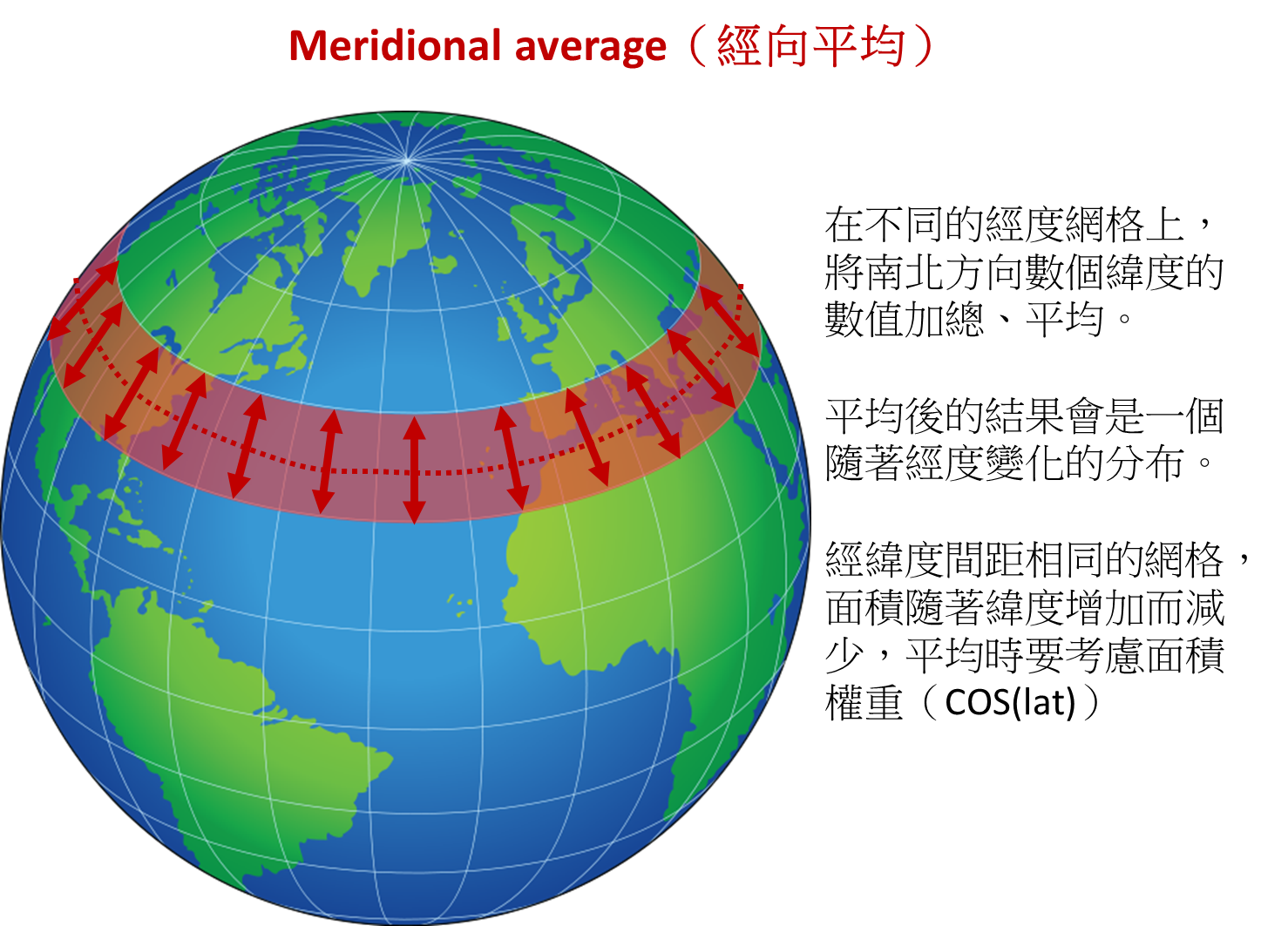
# Ex4. Compute the meridional average T profile

# When doing merional mean (north-south avarage), we need to
# consider the areal weighting of different latitude
wlat=np.cos(np.radians(lat))
plt.plot(lat,wlat)
plt.show()

tma=np.average(t1_3d,axis=1,weights=wlat)
print(tma.shape)

# plot the contour of meridional average T profile
CS=plt.contourf(lon,lev,tma)
plt.colorbar(CS,orientation='vertical')
plt.ylim([1000,1])
plt.title('Meridional mean T, GFS'+date)
plt.show()

# compare with the medional average WITHOUT latitude weighting
tmanoweight=np.average(t1_3d,axis=1)

# plot the first level ([0], 1000 hPa) to show the difference
# The average temperature without weighting is colder, because the Tropical areas (warmer) are under-emphasized
plt.plot(lon,tma[0],'k-',lon,tmanoweight[0],'b-')

plt.legend(['lat weighting','no weighting'])
plt.title('Meridional mean T at 1000 hPa, GFS'+date)
plt.show()
