Python example: Scipy integration 積分工具
這邊介紹使用Scipy.integrate toolbox進行數值積分運算的方法
- Scipy.integrate.quad
- Scipy.integrate.simps
引入要使用的工具庫:Numpy, Scipy, Matplotlib
import numpy as np
import scipy.integrate as integrate # scipy提供的數值積分工具
import matplotlib.pyplot as plt     # for visualization
以下舉例計算積分 $\int_{0}^{10}{x^{2}+1}$
解析解 : $\bigg[\frac{x^{3}}{3}+x\bigg]_0^{10}$=343.3333333333333333333
首先將要積分的函數設成「匿名函數」(anonymous function),語法是
f_name = lambda x : expression
積分的數值範圍(0~10)與間隔0.1用np.linspace設定成陣列
f1 = lambda x : x**2 + 1    # anonymous function to be integrated
xi = np.linspace(0,10,100)  # interval of integration

print(xi[0],f1(xi)[0])   # starting point of the integration (fist element of xi and f1)
print(xi[-1],f1(xi)[-1]) # ending point of the integration (last element of xi and f1)
# Let's visualize the equation and its integration first
plt.plot(xi,f1(xi),'b-')
plt.vlines(xi[0],-10,f1(xi)[0],colors='r')
plt.vlines(xi[-1],-10,f1(xi)[-1],colors='r')
plt.hlines(0,xi[0],xi[-1],colors='r')
plt.xlim(-0.1,10.1)
plt.ylim(0,102)
plt.show()

使用Scipy的積分指令: quad (if the functional form is known)
Integrate A Python function from a to b (possibly infinite interval).
integrate.quad(func, a, b)
- func: funcion name
- a: Lower limit of integration(-np.inf for -infinity)
- b: Upper limit of integration(np.inf for infinity)
回傳:積分值、誤差估計
reference https://docs.scipy.org/doc/scipy/reference/generated/scipy.integrate.quad.html
area = integrate.quad(f1, 0, 10)
print(area)
使用Scipy的積分指令: simpson (if the array to be integrated is known)
Integrate y(x) with sample array x using the Composite Simpson’s rule. If x is not given, spacing of dx is assumed.
integrate.simps(y, x=..., dx=...)
- y: the array to be integrated
- x: the points at which y is sampled.
- dx: Spacing of integration points. Only used when x is None. Default is 1.
reference https://docs.scipy.org/doc/scipy-0.14.0/reference/generated/scipy.integrate.simps.html
integrate.simps(f1(xi),xi)
Composite Simpson's rule: (在大二的數值分析課程會詳細介紹其理論)
https://en.wikipedia.org/wiki/Simpson%27s_rule#Composite_Simpson's_rule
Simply speaking, the Simpson's rule is similar to the trapzoidal rules, but using quadratic polynomials (P(x) below) to approximate the area of a definite integral:
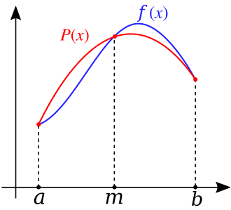
For Composite Simpson's rule, the interval of integration [a,b] is broken into a number of small subintervals (the "x" array). Simpson's rule is then applied to each subinterval, with the results being summed to produce an approximation for the integral over the entire interval.
