# If you use this code to analyze data, please cite the following paper:
# Lin W-Y, Huang C-C, Liu Y-L, Tsai S-J, Kuo P-H (2019). Genome-wide gene-environment interaction analysis with set-based association tests. Frontiers in Genetics, 9, Article 715 (15 pages).
# Any questions or comments, please contact: Wan-Yu Lin, linwy@ntu.edu.tw, Institute of Epidemiology and Preventive Medicine, National Taiwan University College of Public Health
# Thank you.
##########################################################################################
The R code to implement the ADABF GxE method
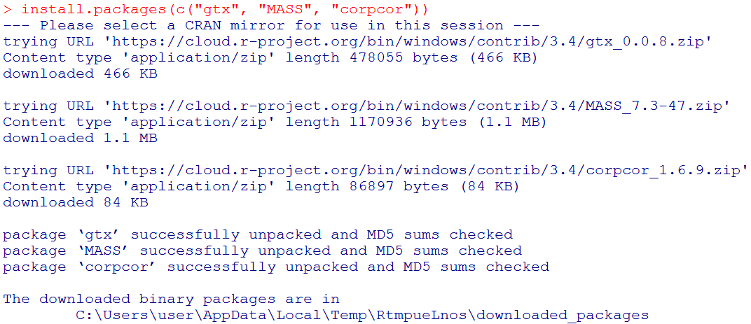
To implement the ADABF method, three R packages, "gtx", "MASS", and "corpcor" need to be installed first.
In R, the code to implement this function is:
source('ADABFGE.R')
ADABFGE(Y, Copy, E, Y.Type="D", E.Type="D", Cov=NULL, Sig=0.05, Precision.P=1)
where Y is the vector of phenotypes,
Copy is the matrix of allele counts (0, 1, 2),
E is the environmental factor,
Y.Type="D" if Y is dichotomous whereas Y.Type="C" if Y is continuous,
E.Type="D" if E is dichotomous whereas E.Type="C" if E is continuous,
and Cov is the matrix of covariates.
Note that the numbers of rows in Copy and Cov are the number of subjects. To know which SNPs enrich the significant GxE signal, we encourage you to provide the SNP names in the header line of Copy. Missing values are represented by the symbol "NA". Sig is the significance level of the gene-based association test. The default significance level of the gene-based association test is set to be 0.05, but it can be changed to other values. Precision.P is the desired precision level of the P-value. Three levels of Precision.P can be specified by the user:
(1) Precision.P=1, the resampling procedure is repeated until the P-value is larger than 10/B, where B is the number of resampling. The number of resampling would be between 102 and 106. This is the default setting, as described in our paper (Page 10 in the PDF file).
(2) Precision.P=2, the resampling procedure is repeated until the P-value is larger than 100/B, where B is the number of resampling. The number of resampling would be between 103 and 107. It takes a longer time than (1).
(3) Precision.P=3, the resampling procedure is repeated until the P-value is larger than 1000/B, where B is the number of resampling. The number of resampling would be between 104 and 108. It takes even a longer time than (2).
Variability of the ADABF P-values: (1) > (2) > (3);
Precision of the ADABF P-values: (3) > (2) > (1);
Time to spend: (3) > (2) > (1).
We provide an example data set:
Dichotomous-trait file
Genotype file
Environmental factor file (Dichotomous)
Environmental factor file (Continuous)
Covariate file
Continuous-trait file
Note that the row ordering of subjects must be consistent among the trait file, genotype file, environmental factor file, and covariate file. Missing values are represented by the symbol "NA".
Please use the following R codes to analyze the dichotomous trait:
Y <- read.table('Dichotomoustrait.txt',header=F)
Copy <- read.table('genotype.txt',header=T) # To know which SNPs enrich the significant association signal, the SNP names are provided in the header line.
En <- read.table('dichoE.txt',header=F)
Cov <- read.table('covariate.txt',header=F)
source('ADABFGE.R')
ADABFGE(Y=Y, Copy=Copy, E=En, Y.Type="D", E.Type="D", Cov=Cov, Sig=0.05, Precision.P=1) # if you want to consider covariates
ADABFGE(Y=Y, Copy=Copy, E=En, Y.Type="D", E.Type="D", Cov=NULL, Sig=0.05, Precision.P=1) # if you do not want to consider covariates
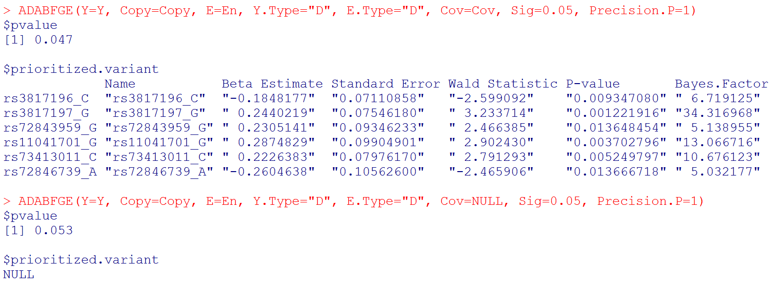
# Output: the P-value of the ADABF test. If the ADABF test is significant, we then prioritize the variants that enrich the significant GxE signal. If the ADABF test is not significant, no variants would be prioritized. The default significance level of the gene-based GxE test is set to be 0.05, but it can be changed to other values.
# Please note that "Beta Estimate" is the minor allele x Environment interaction effect. (Recall that "Copy" is the matrix of allele counts (0, 1, 2), and our R function recodes it to be the matrix of minor allele counts.)
With the sequential resampling approach, the P-value of the ADABF test may vary. If you wish to have a more precise P-value, please use:
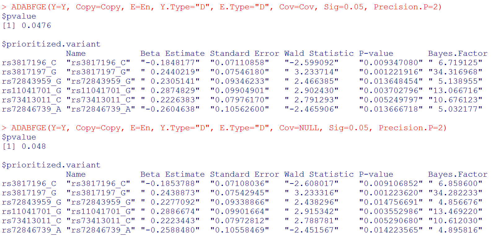
# Please note that "Beta Estimate" is the minor allele x Environment interaction effect. (Recall that "Copy" is the matrix of allele counts (0, 1, 2), and our R function recodes it to be the matrix of minor allele counts.)
Please use the following R codes to analyze the continuous trait:
Y <- read.table('Continuoustrait.txt',header=F)
ADABFGE(Y=Y, Copy=Copy, E=En, Y.Type="C", E.Type="D", Cov=Cov, Sig=0.05, Precision.P=1) # if you want to consider covariates
ADABFGE(Y=Y, Copy=Copy, E=En, Y.Type="C", E.Type="D", Cov=NULL, Sig=0.05, Precision.P=1) # if you do not want to consider covariates
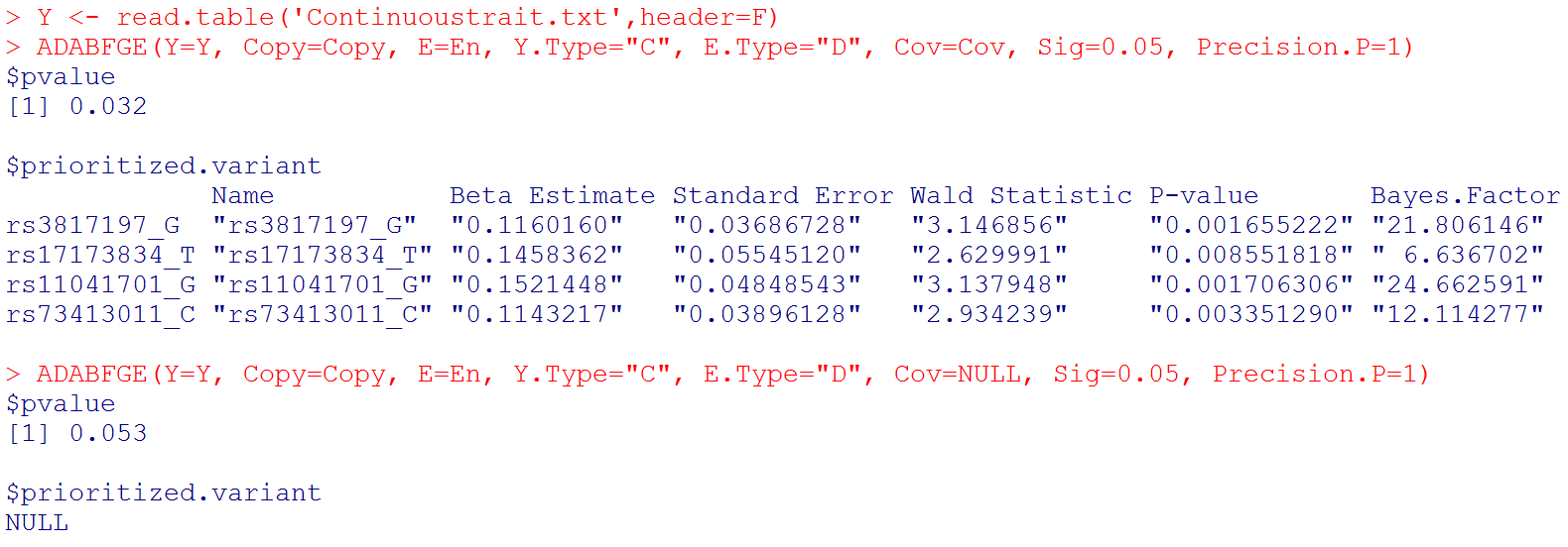
# Output: the P-value of the ADABF test. If the ADABF test is significant, we then prioritize the variants that enrich the significant GxE signal. If the ADABF test is not significant, no variants would be prioritized. The default significance level of the gene-based GxE test is set to be 0.05, but it can be changed to other values.
# Please note that "Beta Estimate" is the minor allele x Environment interaction effect. (Recall that "Copy" is the matrix of allele counts (0, 1, 2), and our R function recodes it to be the matrix of minor allele counts.)
With the sequential resampling approach, the P-value of the ADABF test may vary. If you wish to have a more precise P-value, please use:
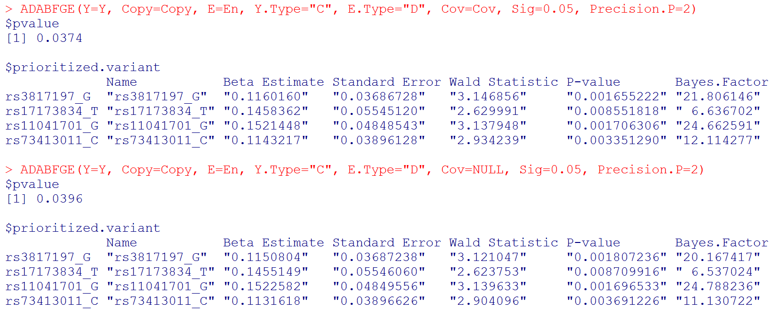
# Please note that "Beta Estimate" is the minor allele x Environment interaction effect. (Recall that "Copy" is the matrix of allele counts (0, 1, 2), and our R function recodes it to be the matrix of minor allele counts.)
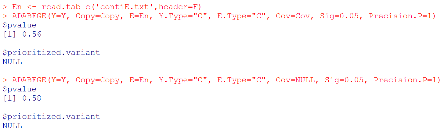
If the environmental factor is continuous, please use the following command:
En <- read.table('contiE.txt',header=F)
ADABFGE(Y=Y, Copy=Copy, E=En, Y.Type="C", E.Type="C", Cov=Cov, Sig=0.05, Precision.P=1) # if you want to consider covariates
ADABFGE(Y=Y, Copy=Copy, E=En, Y.Type="C", E.Type="C", Cov=NULL, Sig=0.05, Precision.P=1) # if you do not want to consider covariates
Thanks for your interest.
How to perform the genome-wide gene-environment interaction analysis?
Return to Wan-Yu Lin's homepage