Adaptive Combination of Bayes Factors (ADABF) Method

##########################################################################################
# A brief introduction: Most gene-based association tests are underpowered given a large proportion of neutral variants within the gene. Our new method, the Adaptive Combination of Bayes Factors (ADABF) Method, removes the variants with smaller Bayes factors and so it is robust to the inclusion of neutral variants. The ADABF method is more powerful than other association tests when there are only few variants (in a gene/region) associated with the phenotypes. It can be applied to GWAS or NGS data, continuous traits or dichotomous traits, unrelated subjects or case-parent trios, and it allows for covariates adjustment. Besides, more than other gene-based association tests, the ADABF method further indicates which variants enrich the significant association signal.

Q: Why the Bayes factor is used to truncate variants, instead of the P-value?

A: The commonly-used P-value is the probability of obtaining a statistic as extreme as or more extreme than the observed statistic under the null hypothesis (H0) of no association. However, a P-value provides no information regarding the alternative hypothesis (H1) and power, which varies with the minor allele frequencies (MAFs). In this work, we show that truncating variants according to P-values is not optimal, when both rare and common variants are considered (please see the subsection “Ranking by Bayes factor vs. P-value”).

# If you use this code to analyze data, please cite the following paper:
# Lin W-Y, Chen W.J., Liu C-M, Hwu H-G, McCarroll S.A., Glatt S.J., Tsuang M.T. (2017). Adaptive combination of Bayes factors as a powerful method for the joint analysis of rare and common variants. Scientific Reports, 7: 13858.     [A poster to briefly introduce this study]
# Any questions or comments, please contact: Wan-Yu Lin, linwy@ntu.edu.tw, Institute of Epidemiology and Preventive Medicine, National Taiwan University College of Public Health
# Thank you.
##########################################################################################

For unrelated subjects:

The R code to implement the ADABF method

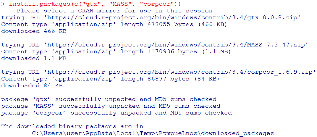
To implement the ADABF method, three R packages, "gtx", "MASS", and "corpcor" need to be installed first.

ADABF_demo1

In R, the code to implement this function is:

source('ADABFunre.R')
ADABFunre(Y, Copy, Type="D", Cov=NULL, Sig=0.05, Precision.P=1)

where Y is the vector of phenotypes, Copy is the matrix of allele counts (0, 1, 2), Type="D" if Y is dichotomous whereas Type="C" if Y is continuous, and Cov is the matrix of covariates. Note that the numbers of rows in Copy and Cov are the number of subjects. To know which SNPs enrich the significant association signal, we encourage you to provide the SNP names in the header line of Copy. Missing values are represented by the symbol "NA". Sig is the significance level of the gene-based association test. The default significance level of the gene-based association test is set to be 0.05, but it can be changed to other values. Precision.P is the desired precision level of the P-value. Three levels of Precision.P can be specified by the user:

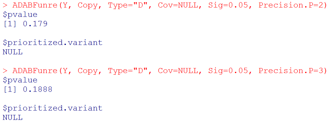
(1) Precision.P=1, the resampling procedure is repeated until the P-value is larger than 10/B, where B is the number of resampling. The number of resampling would be between 10² and 10⁶. This is the default setting, as described in our paper (Page 10 in the PDF file).
(2) Precision.P=2, the resampling procedure is repeated until the P-value is larger than 100/B, where B is the number of resampling. The number of resampling would be between 10³ and 10⁷. It takes a longer time than (1).
(3) Precision.P=3, the resampling procedure is repeated until the P-value is larger than 1000/B, where B is the number of resampling. The number of resampling would be between 10⁴ and 10⁸. It takes even a longer time than (2).

Variability of the ADABF P-values: (1) > (2) > (3);
Precision of the ADABF P-values: (3) > (2) > (1);
Time to spend: (3) > (2) > (1).

We here provide an example data file 'ADABFcscnfile.txt', in which the first column is the disease status (1: case; 0: control), and column 2 to the last column are the numbers of minor alleles. Please use the following R codes to analyze this data set:

Y <- as.matrix(read.table("ADABFcscnfile.txt", header=T))[,1]
Copy <- as.matrix(read.table("ADABFcscnfile.txt", header=T))[,-1]      # To know which SNPs enrich the significant association signal, the SNP names are provided in the header line.
source('ADABFunre.R')
ADABFunre(Y, Copy, Type="D", Cov=NULL, Sig=0.05, Precision.P=1)

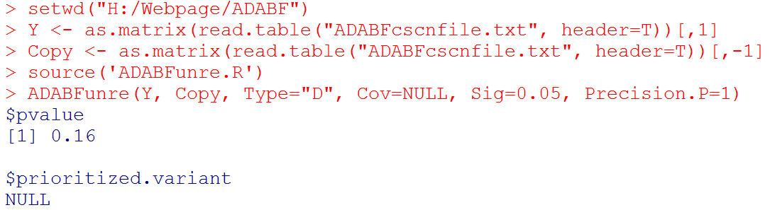
# Output: the P-value of the ADABF test. If the ADABF test is significant, we then prioritize the variants that enrich the significant association signal. If the ADABF test is not significant, no variants would be prioritized. The default significance level of the gene-based association test is set to be 0.05, but it can be changed to other values.

With the sequential resampling approach, the P-value of the ADABF test may vary. If you wish to have a more precise P-value, please use:

We also provide another data set:

Dichotomous-trait file
Genotype file
Covariate file
Continuous-trait file

Note that the row ordering of subjects must be consistent among the trait file, genotype file, and covariate file. Missing values are represented by the symbol "NA".

Please use the following R codes to analyze the dichotomous trait:

Y <- read.table('Dichotomoustrait.txt',header=F)
Copy <- read.table('genotype.txt',header=T)     # To know which SNPs enrich the significant association signal, the SNP names are provided in the header line.
Cov <- read.table('covariate.txt',header=F)
source('ADABFunre.R')
ADABFunre(Y, Copy, Type="D", Cov=Cov, Sig=0.05, Precision.P=1)       # if you want to consider covariates
ADABFunre(Y, Copy, Type="D", Cov=NULL, Sig=0.05, Precision.P=1)     # if you do not want to consider covariates

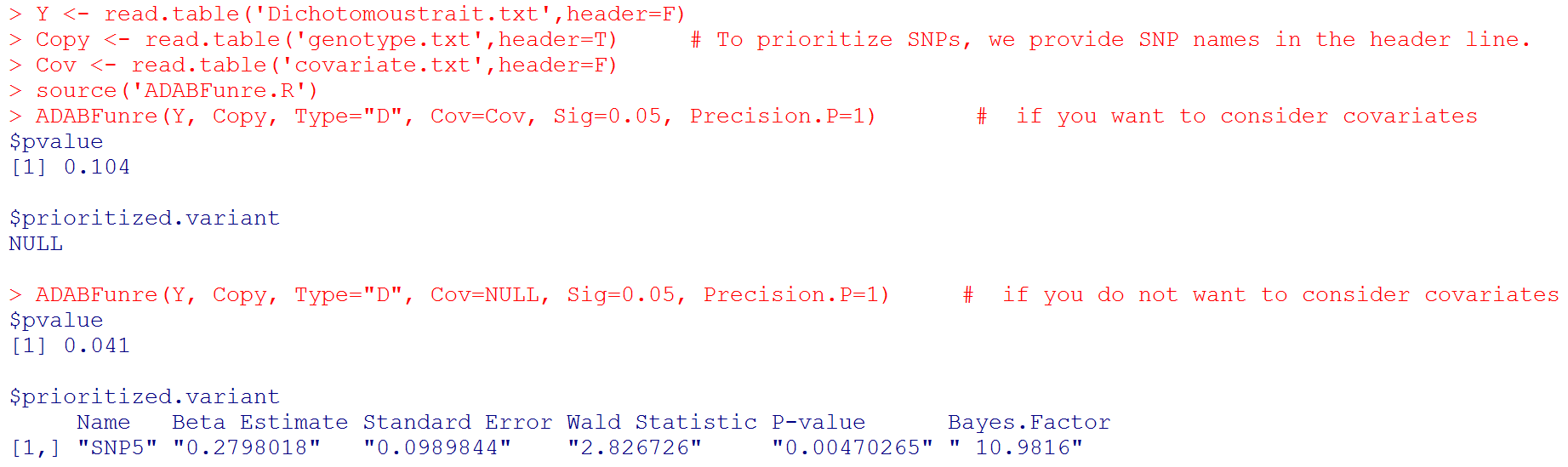
# Output: the P-value of the ADABF test. If the ADABF test is significant, we then prioritize the variants that enrich the significant association signal. In the bottom example, the variant "SNP5" is prioritized. If the ADABF test is not significant, no variants would be prioritized. The default significance level of the gene-based association test is set to be 0.05, but it can be changed to other values.

# Please note that "Beta Estimate" is the effect of minor allele. (Recall that "Copy" is the matrix of allele counts (0, 1, 2), and our R function recodes it to be the matrix of minor allele counts.)

With the sequential resampling approach, the P-value of the ADABF test may vary. If you wish to have a more precise P-value, please use:

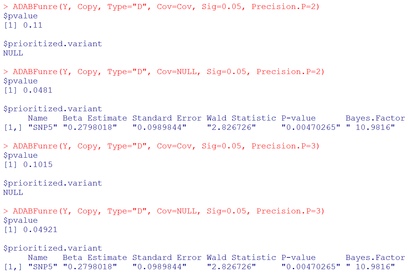
# Please note that "Beta Estimate" is the effect of minor allele. (Recall that "Copy" is the matrix of allele counts (0, 1, 2), and our R function recodes it to be the matrix of minor allele counts.)

Please use the following R codes to analyze the continuous trait:

Y <- read.table('Continuoustrait.txt',header=F)
ADABFunre(Y, Copy, Type="C", Cov=Cov, Sig=0.05, Precision.P=1)       # if you want to consider covariates
ADABFunre(Y, Copy, Type="C", Cov=NULL, Sig=0.05, Precision.P=1)     # if you do not want to consider covariates

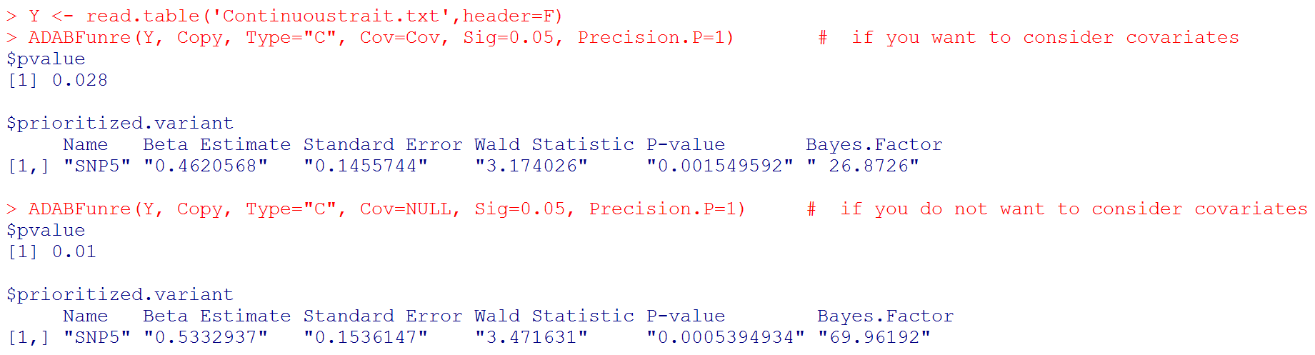
# Output: the P-value of the ADABF test. If the ADABF test is significant, we then prioritize the variants that enrich the significant association signal. In these two examples, the variant "SNP5" is prioritized. If the ADABF test is not significant, no variants would be prioritized. The default significance level of the gene-based association test is set to be 0.05, but it can be changed to other values.

# Please note that "Beta Estimate" is the effect of minor allele. (Recall that "Copy" is the matrix of allele counts (0, 1, 2), and our R function recodes it to be the matrix of minor allele counts.)

With the sequential resampling approach, the P-value of the ADABF test may vary. If you wish to have a more precise P-value, please use:

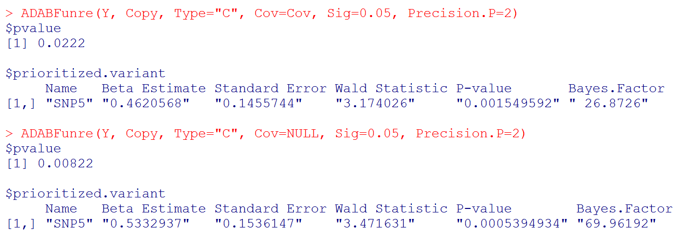
# Please note that "Beta Estimate" is the effect of minor allele. (Recall that "Copy" is the matrix of allele counts (0, 1, 2), and our R function recodes it to be the matrix of minor allele counts.)

For case-parent trios:

The R code to implement the ADABF method

In R, the code to implement this function is:    (the R packages "gtx", "MASS", and "corpcor" need to be installed first)

source('ADABFtrios.R')
ADABFtrios(Copytrio, Sig=0.05, Precision.P=1)

where Copytrio is the matrix of allele counts (0, 1, 2), in which the first 1/3 rows are the genotypes of the affected children, the second 1/3 rows are the genotypes of mothers, and the last 1/3 rows are the genotypes of fathers. Missing values are represented by the symbol "NA". To know which SNPs enrich the significant association signal, we encourage you to provide the SNP names in the header line of Copytrio. Sig is the significance level of the gene-based association test. The default significance level of the gene-based association test is set to be 0.05, but it can be changed to other values. Precision.P is the desired precision level of the P-value. Three levels of Precision.P can be specified by the user:

(1) Precision.P=1, the resampling procedure is repeated until the P-value is larger than 10/B, where B is the number of resampling. The number of resampling would be between 10² and 10⁶. This is the default setting, as described in our paper (Page 10 in the PDF file).
(2) Precision.P=2, the resampling procedure is repeated until the P-value is larger than 100/B, where B is the number of resampling. The number of resampling would be between 10³ and 10⁷. It takes a longer time than (1).
(3) Precision.P=3, the resampling procedure is repeated until the P-value is larger than 1000/B, where B is the number of resampling. The number of resampling would be between 10⁴ and 10⁸. It takes even a longer time than (2).

Variability of the ADABF P-values: (1) > (2) > (3);
Precision of the ADABF P-values: (3) > (2) > (1);
Time to spend: (3) > (2) > (1).

We here provide an example data file 'ADABFtriosfile.txt' . Please use the following R codes to analyze this data set:

source('ADABFtrios.R')
Copytrio <- as.matrix(read.table("ADABFtriosfile.txt", header=T))     # To know which SNPs enrich the significant association signal, the SNP names are provided in the header line.
ADABFtrios(Copytrio, Sig=0.05, Precision.P=1)

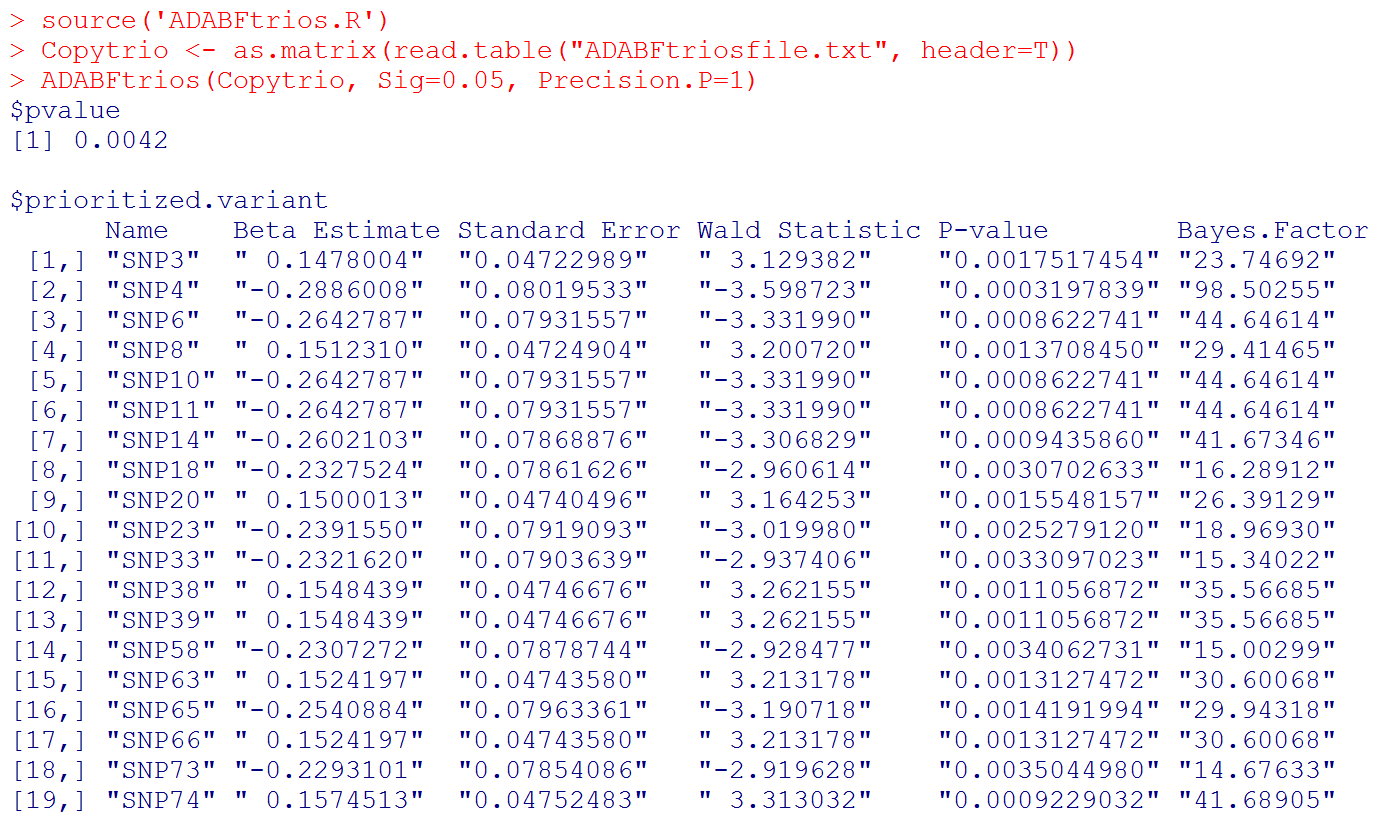
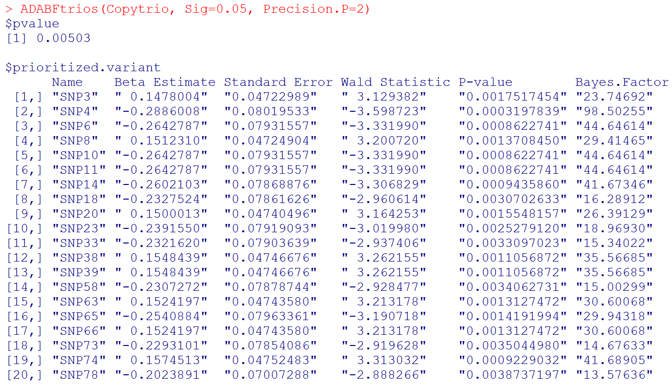
# Output: the P-value of the ADABF test. If the ADABF test is significant, we then prioritize the variants that enrich the significant association signal. In this example, the variants "SNP3", ..., "SNP74" are prioritized. If the ADABF test is not significant, no variants would be prioritized. The default significance level of the gene-based association test is set to be 0.05, but it can be changed to other values.

# Please note that "Beta Estimate" is the effect of minor allele. (Recall that "Copy" is the matrix of allele counts (0, 1, 2), and our R function recodes it to be the matrix of minor allele counts.)

With the sequential resampling approach, the P-value of the ADABF test may vary. If you wish to have a more precise P-value, please use: